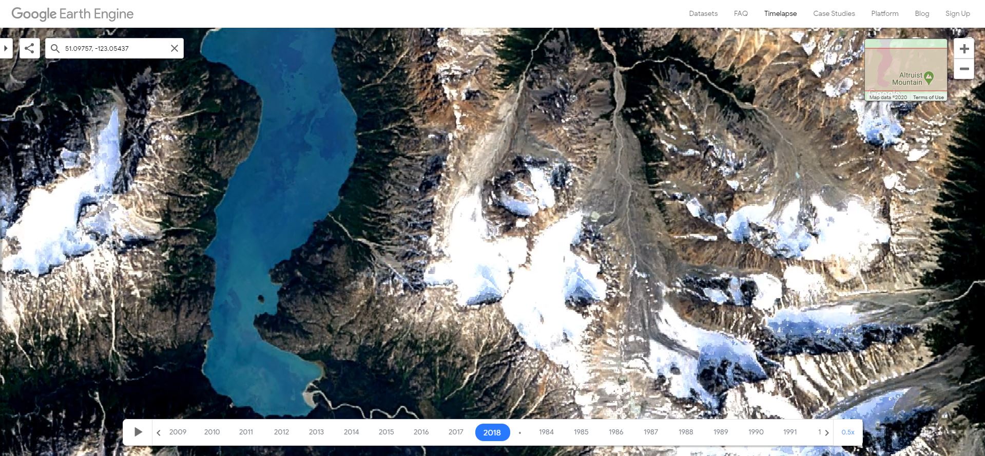
Step 1: Capture Google Earth Engine Timelapse imagery (Figures EX2.1 & EX2.2).

1. Visit Google Earth Engine Timelapse and navigate to a large scale view of your glacier. It may load slowly, so give it a few moments. Zoom in as far as possible with your glacier in the centre of the view. Press the pause button on the lower left of the screen, then choose the earliest view (e.g., 1984) where the position of the toe of your glacier is visible. The earliest view should be before 1990.
2. Create a screen capture of this view and save it with the file name <5_Lastname 1984 imagery>. Add the image to your document as Figure EX2.1.
3. Write a caption for Figure EX2.1 indicating what the image is of, the date of the imagery and include a link to this view by using the Share Current View button and pasting it as the image source.
4. Keeping the exact same view, repeat the previous three steps to produce Figure EX2.2 using the most recent imagery and save the screen capture with the file name <6_year_Lastname_Glacier_extent>. Figure 22.5 provides an example. Write a caption for Figure EX2.2 describing any changes you observe.

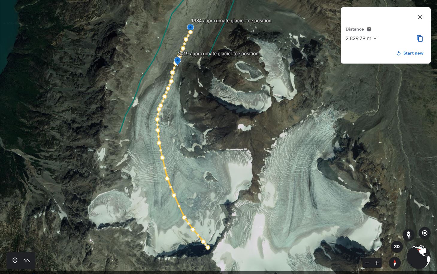
Step 2: Estimate the approximate location of the glacier toe in 1984 (creating a point feature and Figure EX2.3).

1. Using landmarks visible in the earliest good imagery from Google Earth Engine Timelapse (this will most likely  be 1984), add a point feature to your Google Earth project and move it to your best estimate of the location of the toe of the glacier in 1984. Use as many landmarks as possible to situate your point. Make sure your view is in 2D and it helps if you view both images at the same scale.
2. For comparison, measure the length of the glacier you estimate in 1984 and create a screen capture of your measurement while the value of the measurement is still visible. Save this screen capture of Google Earth (Web) as <7_Lastname_1984_approximate_glacier_toe> (example provided as Figure 22.6).

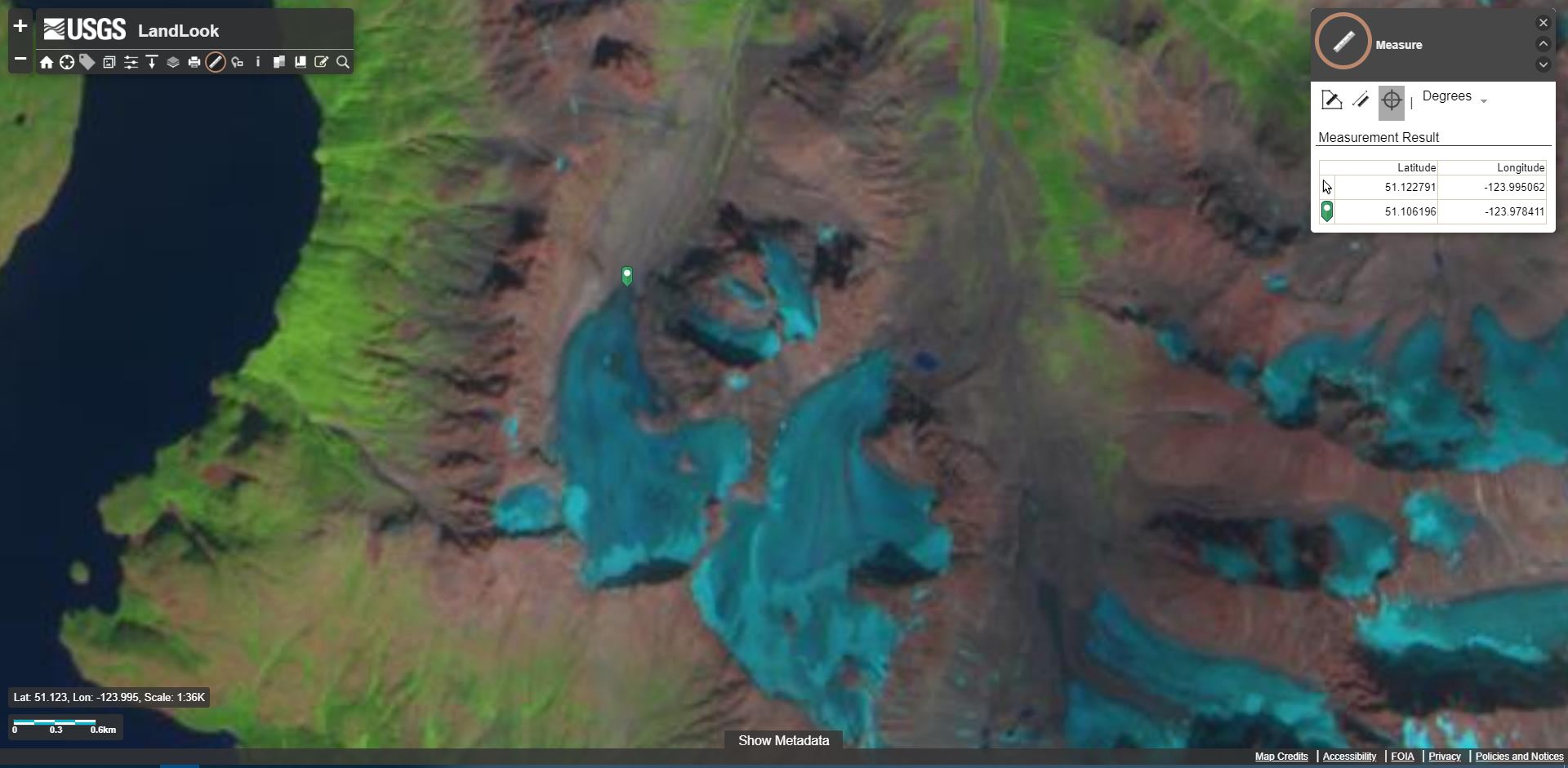
Step 3: Analyze the accumulation zone in the most recent satellite imagery (Figure EX2.4).

1. Go to the USGS LandLook website tool for viewing recent satellite imagery and navigate to a large scale view of your glacier.
2. View your chosen glacier by typing in the coordinates of your glacier or name of your glacier in the search pane (magnifying glass icon) and zoom in until the glacier fills a lot of your map area.
3. Set the menu so that only Sentinel 2 MSI (2015-Present) displays by only having the box of this type of imagery set.
4. In order to find the date of the best Sentinel 2 MSI (2015-present) image capturing the most recent size and pattern of the true accumulation zone, set the year to start from and extend to only the most recent year that there is 12 months of data.  For instance, if you are doing this lab in Fall 2025, you will need to use the 2024 images.
5. Modify the Days of the Year in the search pane so that results display the size and pattern of the true accumulation zone. This date coincides with the time of year when the size of the preserved snowpack from the previous winter will be at a minimum. Therefore, set the date range for your search to mid or late summer. For glaciers in low latitudes (southern and central BC or Alberta), set the Days of the Year from early August to late September. For glaciers in higher latitudes (Yukon, Nunavut and northern BC or Alberta) set the dates from early July to Late August. Video 22.2 provides instructions on how to do this.

Video 22.2. How to Search and Download Satellite Imagery. Real-time closed captioning and transcript are available on YouTube.

6. Once the images are loaded (this might take some time), ensure that you turn the Dynamic Image Refresh off in the Image Display menu. Press the play button (black triangle) until you find the best scene depicting the minimum size of the accumulation zone. Press stop (black square) at this image. Record the image’s date (written directly below where it says Active Date in bold letters; e.g., August 27th, 2024).
7. Using the Measure tool and then Location button (circle with a cross over it) record the geographic grid coordinates in decimal degrees of the glacier toe. Once you have clicked the location, the coordinate appears in a table beside the green placemark icon.
8. Record the position.
9. Create a screen capture of the glacier and save it in a file named <8_Lastname_daymonthyear_Sentinel_2_image>.
10. Add this file to your document as Figure EX2.4 (refer to Figure 22.7 for an example) and indicate the image source by adding the URL of your current view.  Do this by using the Bookmarks button then Generate URL button.
11. Write a caption in which you describe and discuss the following questions:

    a. What is the likelihood of the glacier disappearing in the current climate regime? Please refer to the visual evidence described in the lab introduction that supports your prediction.

    b. What observations are you basing your hypothesis on? This involves describing the visual evidence you used.

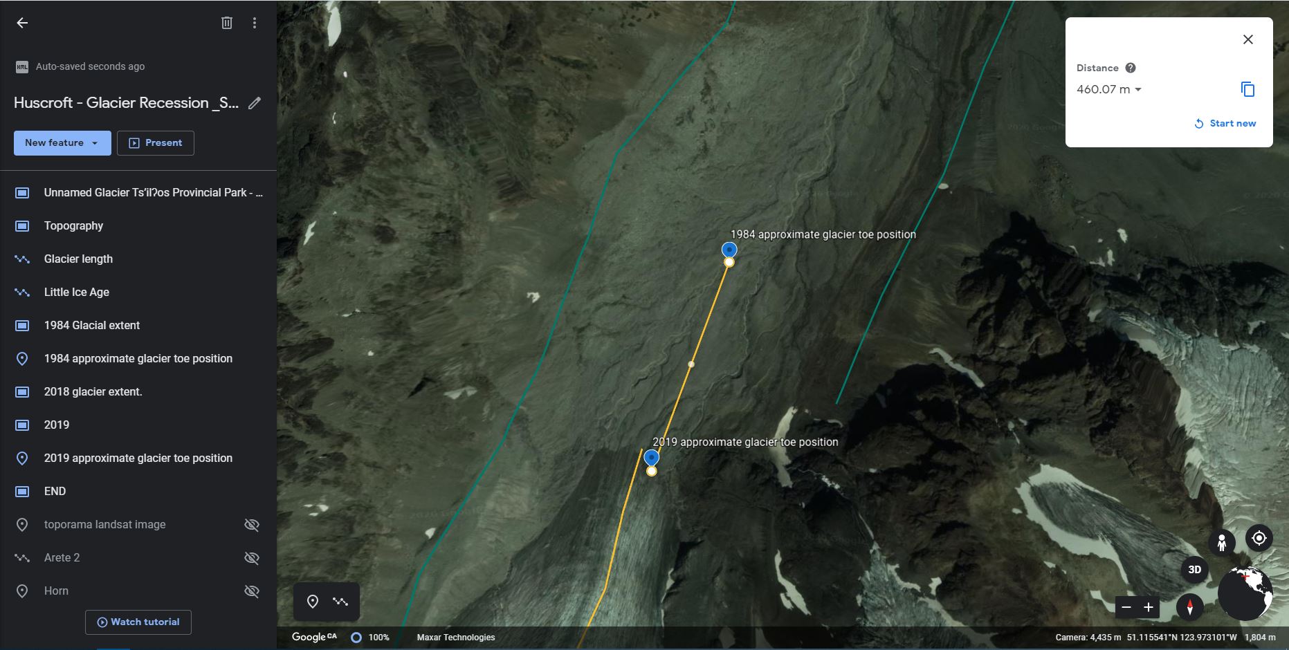
Step 4: Calculate the rate of change (Figure EX2.5).

1. Using the coordinates recorded in the previous step, add a point to your Google Earth (Web) project called <Year approximate glacier toe position>. For example, 2024 approximate glacier toe position.
2. Measure the distance between this location and the 1984 position and calculate the average rate of retreat or advance of the glacier. Take a screen capture of this measurement and save the measurement as <9_Lastname_glacier_position_measurement>.  Add this image to your document as Figure EX2.5. An example is provided as Figure 22.8.
3. Write a caption that includes the total measured retreat (or advance) distance over the period from your earliest photo until the most recent satellite imagery, and the average rate of retreat.

Step 5: Get curious and do a small scientific analysis of your own choosing.

1. By exploring the tools and images available to you on the websites you have used so far in this lab, do an extra analysis of your own creation and add extra screen capture(s) as figure(s) that support your analysis as Figure EX2.6 (and additional if needed). Try to keep it as simple as possible. Be sure to state the question you are trying to answer in your analysis as well as your method. Possible analyses could involve:

• • Doing an extra measurement.
  • Accessing imagery from a different time and doing comparisons.
  • Finding imagery on the The Atlas of Canada – Toporama website or the iMap BC website and comparing glacier toe positions.

1. Review your text for grammatical and spelling mistakes.
2. Export your document to a PDF. Your PDF file needs to be a reasonable size (generally less than 5MB, but ask your lab instructor for details). In order to do this, you will need to reduce (compress) the file size of all of your images to between 150-100 ppi. Be sure to check that you have not compressed the images so much that you are not able to see them clearly on your monitor. For PC users, the compression can be done with MSWord by clicking on the image, choosing Picture Tools – Compress.

Submit as directed by your instructor.

References

GISGeography. (Last updated 2021, February 27). 5 Free Historical Imagery Viewers to Leap Back in the Past. https://gisgeography.com/free-historical-imagery-viewers/
Pelto, M. S. (2010). Forecasting temperate alpine glacier survival from accumulation zone observations. The Cryosphere 4, 67–75. https://doi.org/10.5194/tc-4-67-2010